
Alex Neill, 2015
As explained in the short article Types of numbers there are several different categories of numbers that students are introduced to when working mathematically.
The type of number used is particularly important when dealing with algebraic patterns and relationships, as they influence how a pattern or relationship is represented and interpreted.
The type of number used is particularly important when dealing with algebraic patterns and relationships, as they influence how a pattern or relationship is represented and interpreted.
Two examples: They look the same, but are they?
The following two examples look similar, but there is a fundamental difference between them. Can you spot it?
|
Example 1 - Stick patterns and rules
(http://arbs.nzcer.org.nz/resources/stick-patterns-and-rules)
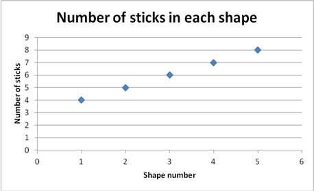
These shapes are made up from ice block sticks. 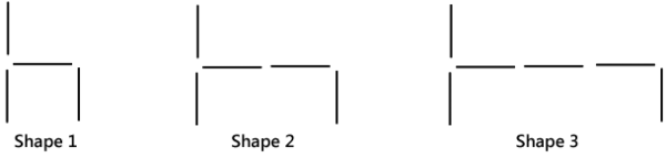
Complete this table to show how many matches will be in Shapes 4 and 5.
 |
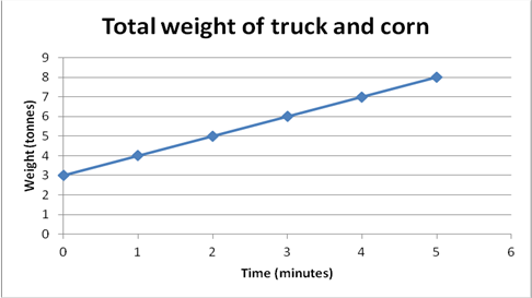
Example 2 - A truck is being filled with corn at a steady rate.
Complete this table of the total weight of the truck and corn after 4 and 5 minutes.
 |
|
Answer:
Example 1 only deals with the numbers 1, 2, 3, 4, ... etc. for both the shape number and the number of sticks. These numbers are called the natural numbers or counting numbers. They are discrete, which means that they go in distinct jumps, with no other natural numbers in between. For example, there is no natural number between 2 and 3. This stick pattern is an example of a sequence.
|
Answer:
Example 2 can use any positive number. The weight could be anything (e.g., 4.36 tonnes), and the time could be in parts of a minute ( e.g., 1.36 minutes). Both weight and time are examples of real numbers. They are continuous numbers because there are an infinite number of other real numbers between any two real numbers, which means that real numbers increase smoothly.
|
For more about discrete and continuous numbers, click on Types of data: Statistics or Types of numbers.
More about sequences
- A sequence is a collection of objects (also called members) which have a given order. The order is described using the ordinal numbers 1st, 2nd, 3rd, 4th, 5th, etc. Example 1 is the sequence (4, 5, 6, 7, ...), with "4" as the 1st member, "5" the 2nd, etc.
- Students often start off by learning about sequences of shapes, sounds or colours. The Algebraic Patterns Concept Map gives a wealth of information about sequences.
- A sequence may have a fixed length, in which case we call it finite — for example (10, 20, 30, 40) has just 4 members. We want, however, to move students onto sequences that go on forever, such as (1, 3, 5, 7, 9, ...) — the odd numbers. This is an infinite sequence as it has an infinite number of members. We can still count it, so we say that it is countably infinite.
NOTE: Sequences are not an ideal way to introduce the idea of an intercept. An intercept is where a graph crosses the y-axis (i.e., the vertical axis). The next section shows this.
Major differences between the examples
|
Example 1
 |
Example 2
 |
|
|
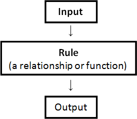
About relationships and functions
One way of thinking about relationships is that they are like a machine. The machine takes some inputs and has a rule that gives some outputs.
|
Examples:
Discrete numbers - recursive rules These give the relationship between successive output numbers
|
 |
Students typically begin with recursive rules, then move on to functional rules. For more go to the Algebraic patterns concept map.
The resource Graphing relationships shows an example of a relationship between two numerical variables. It is represented by ordered pairs plotted on a Cartesian plane.
In the ARBs, we mostly use relationships where the inputs and outputs are numbers, and where a single input number gives a single output number. These relationships are called one-to-one relationships or functions. The input and output are often written as an ordered pair, e.g., (4, 7).